
Cambium 2022 Scenario Descriptions and Documentation
/Pieter Gagnon, Brady Cowiestoll, and Marty Schwarz
National Renewable Energy Laboratory
Cambium 2022 Scenario Descriptions and Documentation
Pieter Gagnon, Brady Cowiestoll, and Marty Schwarz
National Renewable Energy Laboratory
Suggested Citation:
Gagnon, Pieter, Brady Cowiestoll, and Marty Schwarz. 2023. Cambium 2022 Scenario Descriptions and Documentation. Golden, CO: National Renewable Energy Laboratory. NREL/TP-6A40-84916. https://www.nrel.gov/docs/fy23osti/84916.pdf.
Acknowledgments
We gratefully acknowledge the many individuals whose efforts contributed to this work. We thank Mike Meshek for editing the manuscript. We are grateful for the conversations with Matt Clouse, Wesley Cole, Beth Conlin, Olivier Corradi, Hallie Cramer, James Critchfield, Charles Eley, Ellen Franconi, Elaine Hale, Joshua Kneifel, Cara Marcy, Greg Miller, Dev Millstein, Gian Porro, Michael Sontag, Paul Spitsen, and Colby Tucker, whose insights and feedback have proven invaluable when assembling this product. We also thank James Morris and Jianli Gu for maintaining the online scenario viewer that makes dissemination of this work possible. This report was funded by the DOE Office of Energy Efficiency and Renewable Energy under contract number DE-AC36-08GO28308. Any errors or omissions are the sole responsibility of the authors.

1. Cambium Overview
The ReEDS reduced-form dispatch, aided by Augur’s parameterization, aims to capture enough operational detail for realistic bulk power system investment and retirement decisions, but it does not have the temporal resolution that is desired for Cambium databases. To obtain more-detailed simulations of the electric systems projected by ReEDS, NREL developed utilities to represent a ReEDS capacity expansion solution in the second of the two models that Cambium draws from: PLEXOS (Energy Exemplar 2019).
PLEXOS is a commercial production cost model that can simulate least-cost hourly dispatch of a set of generators with a network of nodes and transmission lines. It incorporates representations of unit-commitment decisions, detailed operating constraints (e.g., maximum ramp rates and minimum generation levels), and operating reserves; and it can be run with nested receding horizon planning periods (e.g., day-ahead and real-time) to simulate realistic electric system operations.
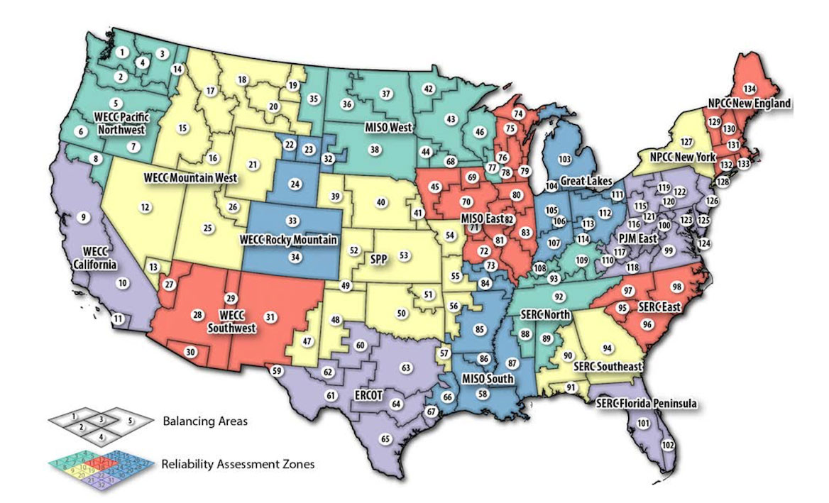
For representing a ReEDS solution as a PLEXOS model, the spatial resolution from ReEDS is retained: the 134 BAs in ReEDS are represented as transmission nodes in PLEXOS, and the connections between them are modeled using the line capacities and loss rates in the ReEDS
1.1 ReEDS
The ReEDS reduced-form dispatch, aided by Augur’s parameterization, aims to capture enough operational detail for realistic bulk power system investment and retirement decisions, but it does not have the temporal resolution that is desired for Cambium databases. To obtain more-detailed simulations of the electric systems projected by ReEDS, NREL developed utilities to represent a ReEDS capacity expansion solution in the second of the two models that Cambium draws from: PLEXOS (Energy Exemplar 2019).
PLEXOS is a commercial production cost model that can simulate least-cost hourly dispatch of a set of generators with a network of nodes and transmission lines. It incorporates representations of unit-commitment decisions, detailed operating constraints (e.g., maximum ramp rates and minimum generation levels), and operating reserves; and it can be run with nested receding horizon planning periods (e.g., day-ahead and real-time) to simulate realistic electric system operations.
For representing a ReEDS solution as a PLEXOS model, the spatial resolution from ReEDS is retained: the 134 BAs in ReEDS are represented as transmission nodes in PLEXOS, and the connections between them are modeled using the line capacities and loss rates in the ReEDS.
1.2 PLEXOS
The ReEDS reduced-form dispatch, aided by Augur’s parameterization, aims to capture enough operational detail for realistic bulk power system investment and retirement decisions, but it does not have the temporal resolution that is desired for Cambium databases. To obtain more-detailed simulations of the electric systems projected by ReEDS, NREL developed utilities to represent a ReEDS capacity expansion solution in the second of the two models that Cambium draws from: PLEXOS (Energy Exemplar 2019).
PLEXOS is a commercial production cost model that can simulate least-cost hourly dispatch of a set of generators with a network of nodes and transmission lines. It incorporates representations of unit-commitment decisions, detailed operating constraints (e.g., maximum ramp rates and minimum generation levels), and operating reserves; and it can be run with nested receding horizon planning periods (e.g., day-ahead and real-time) to simulate realistic electric system operations.
For representing a ReEDS solution as a PLEXOS model, the spatial resolution from ReEDS is retained: the 134 BAs in ReEDS are represented as transmission nodes in PLEXOS, and the connections between them are modeled using the line capacities and loss rates in the ReEDS aggregated transmission representation. Generation capacity at each node is, however, converted from aggregate ReEDS capacity to individual generators using a characteristic unit size for each technology. For consistency, ReEDS cost and performance parameters are used when possible and reasonable, but values derived from previous NREL studies (e.g., Lew et al. [2013]) are used when parameters are unavailable from ReEDS or are available but unreasonable because of structural differences between the models.
Once the ReEDS solution is converted to a PLEXOS database, the hourly dispatch of the grid can be simulated for a full year. For Cambium databases, we run PLEXOS as a mixed integer program, with day-ahead unit commitment and dispatch (without any real-time adjustments for subhourly dispatch or forecast error). For each modeled year, generators have constant heat rates and maximum generator output. Generator short-run marginal costs (SRMC) are generally constant across the year, except for natural gas powered generators, whose SRMC changes with monthly variations in natural gas prices. Supply and demand are balanced at the busbar level, and distribution losses are captured in data pre- and post-processing, as described in Section 6.7. Inter-BA transmission is represented as pipe flow with constant loss rates, with no intra-BA transmission losses. Generator outages are represented by derating installed capacity to an effective capacity based on annual average outage rates that vary by technology. Three operating reserves are represented—regulation, flexibility, and spinning reserves—as detailed in Section 6.10.
We draw from these simulated results—from both ReEDS and PLEXOS—to calculate the metrics reported within Cambium databases, with varying degrees of post-processing, as described in the remainder of this document.
2 User Guidance, Caveats, and Limitations of Cambium Databases
When projecting the expansion and operation of the U.S. electric system in coming decades, it is necessary to make various simplifications. Here, we list some important limitations and caveats that result from these simplifications:
- Cambium Data Should Not Be the Sole Basis for Decisions: Cambium data sets contain modeled projections of the future under a range of possible scenarios. Although we strive to capture relevant phenomena as comprehensively as possible, the models used to create the data are unavoidably imperfect, and the future is highly uncertain. Consequentially, these data should not be used as the sole basis for making decisions. In addition to drawing from multiple scenarios within a single Cambium set, we encourage analysts to draw on projections or perspectives from other sources, to benefit from diverse analytical frameworks when forming their conclusions about the future of the power sector.
- Cambium’s Metrics are Derived from System-Wide, Cost-Minimizing Optimization Models: The models that Cambium draws from take system-wide, cost-minimizing perspectives that do not necessarily reflect the decision-making of individual actors, whose actions may not align with system-wide cost-minimization because of differing incentives or information deficits.
- The Spatial and Temporal Resolution of the Underlying Models is Coarse: Though the models that Cambium draws from have high spatial and temporal resolution for models of their scope, they do require simplifications and aggregations along those dimensions.6 Perhaps most critically, the United States is represented as 134 “copperplate” balancing areas (BA). This lack of transmission losses and constraints within BAs tends to produce lower and less variable marginal costs than what is observed in practice.
- Cambium Reports Marginal Costs, Which Can Differ from Market Prices: Cambium databases contain estimates of various marginal costs (i.e., how much the costs of building and operating the power sector increases with an increase in demand). Importantly, market prices in practice can deviate from marginal costs due to market design, contract structures, cost recovery for nonvariable costs, and bidding strategies. We strongly encourage users to read the descriptions of each marginal cost metric reported in Cambium (Section 5.6) for an understanding of the limitations of each metric.
- Cambium’s Marginal Costs are Not Estimates of Retail Rates: The marginal costs in Cambium should not be directly used as estimates of retail electricity prices because (1) retail rates typically include cost recovery for administrative, distribution infrastructure, and other expenses that are not represented in Cambium databases and (2) retail rates are often set through a ratemaking process that, while sometimes reflecting temporal patternsin the marginal costs of electricity, are generally not priced directly at marginal costs but rather seek to balance cost-recovery, equity, and cost-causation.
- The Full Range of Uncertainty is Not Captured: The models that Cambium draws from compute deterministic least-cost solutions for a particular set of assumptions—each scenario, therefore, does not fully reflect the uncertainties in the underlying assumptions and data. Cambium, through the Standard Scenarios, tries to address this by providing a suite of possible futures, although the full range of possible outcomes can never be fully captured; for example, no scenario includes a severe economic depression as one of many possible futures that are not modeled.
- Cambium is Not Designed to Assess Grid Reliability or Resource Adequacy: Although the models that Cambium draws from can recognize dropped load when insufficient capacity is available to meet demand, these runs should not be considered as assessing grid reliability or resource adequacy, because, among other reasons, (1) only a specific set of conditions (weather, load, and renewable resource quality) is simulated, (2) important temperature effects on generator efficiencies and transmission losses are not represented, (3) transmission line outages are not represented, and (4) intra-BA transmission line constraints are not captured.
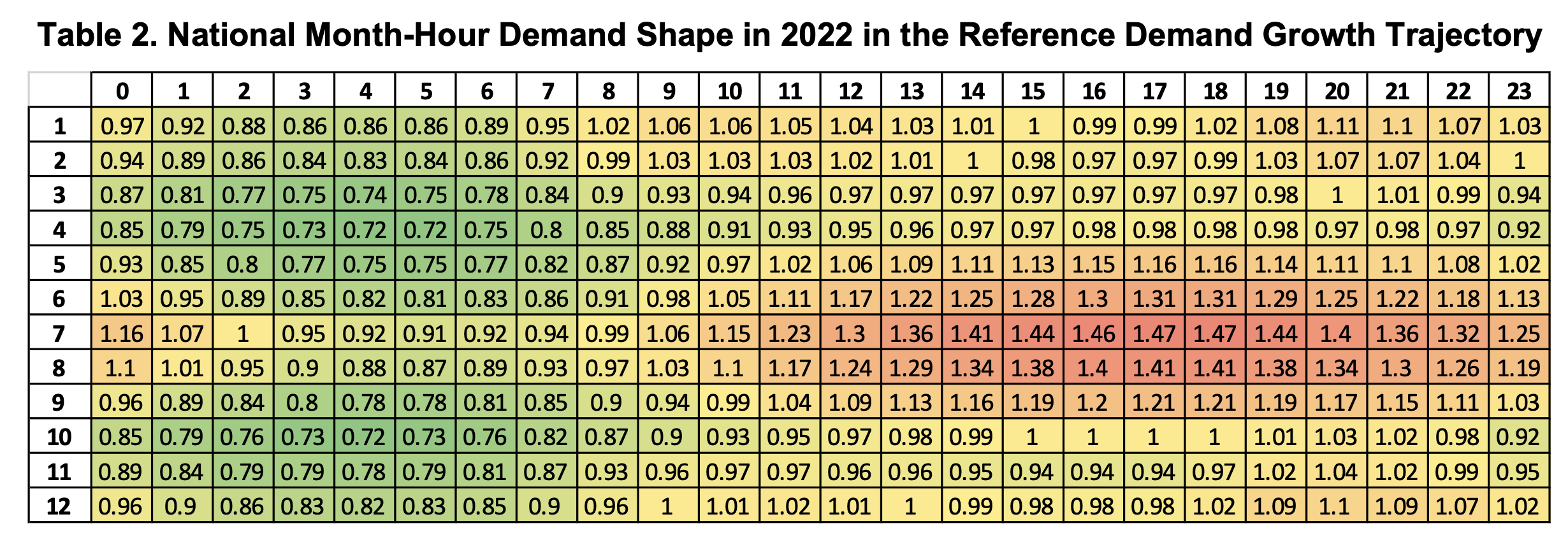
3.0 Demand Growth and Flexibility
The base set of assumptions use a demand growth trajectory that is meant to reflect light electrification induced in part by the demand-side provisions of IRA. The trajectory was created by taking the Medium Electrification scenario from the Electrification Futures Study (Mai et al. 2018) and reducing the rate of electricity growth such that the original values that were reached in 2046 are instead reached in 2050. This rate of growth was selected such that the level of electrification in 2050 was approximately halfway between the AEO2022 (EIA 2022) Reference case and the original Medium Electrification scenario. We emphasize that this is only a simple estimate and that users should look to forthcoming work from NREL and others that develops more-sophisticated estimates of future demand growth.
The high demand growth scenario is the High Electrification with Moderate end-use technology advancement scenario from the Electrification Futures Study (Jadun et al. 2017). The demand trajectories have compound annual growth rates of 1.27% and 1.99% from 2022 through 2050. We assume inelastic, inflexible electricity demand in all scenarios.

4.0 Fuel Prices
Natural gas input price points are based on the trajectories from AEO2022 (EIA 2022). The input price points are drawn from the AEO2022 Reference scenario, the AEO2022 Low Oil and Gas Supply scenario, and the AEO2022 High Oil and Gas Supply scenario (EIA 2022). Actual natural gas prices in ReEDS are based on the AEO scenarios, but they are not exactly the same; instead, they are price-responsive to ReEDS natural gas demand in the electric sector. Each census region includes a natural gas supply curve that adjusts the natural gas input price based on both regional and national demand (Cole, Medlock III, and Jani 2016). Figure 2 shows the output natural gas prices from the suite of scenarios.
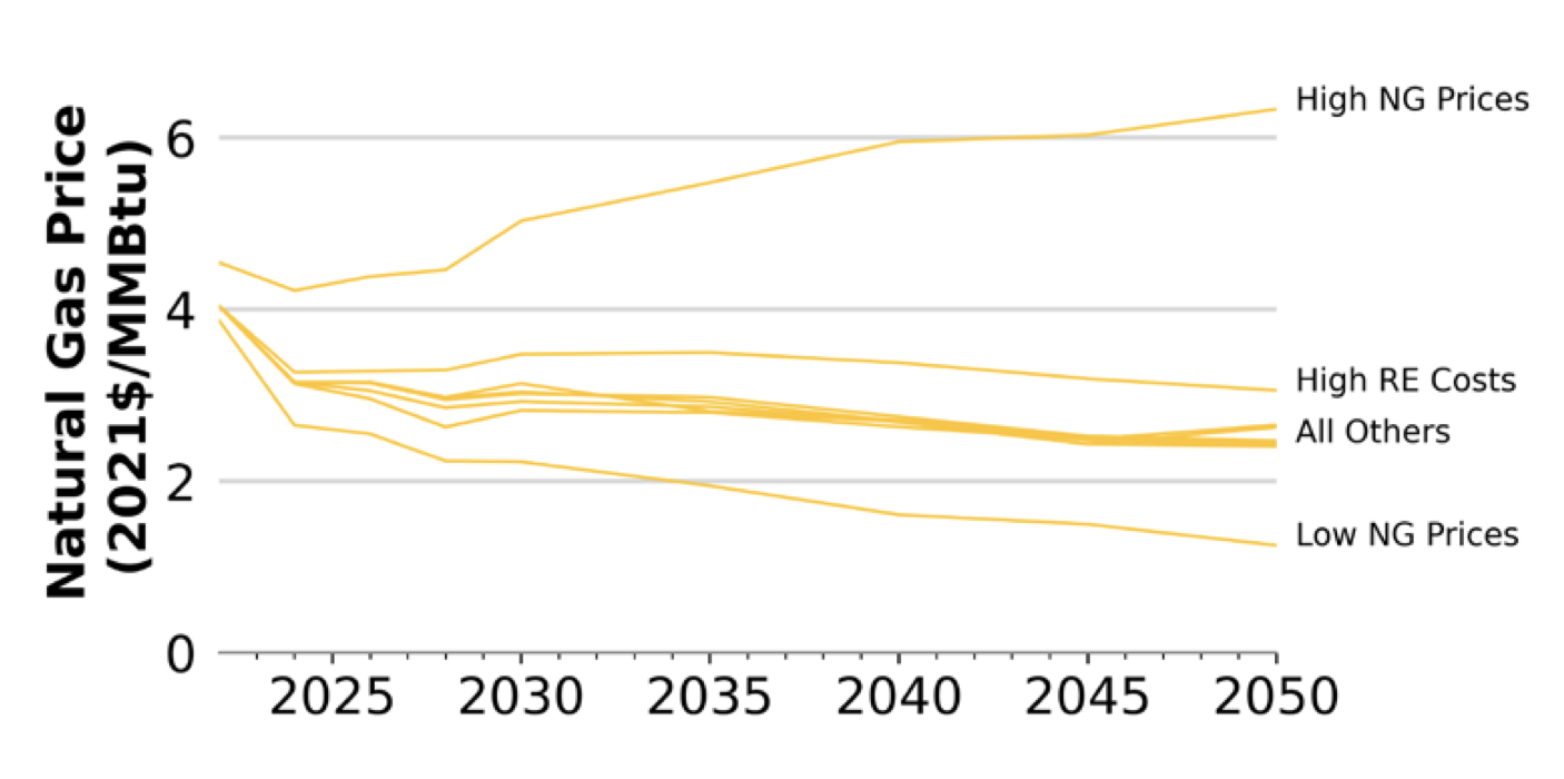
National average natural gas price outputs from the suite of scenarios
The coal and uranium price trajectories are from the AEO2022 Reference scenario and are shown in Figure 3. Both coal and uranium prices are assumed to be fully inelastic. Coal prices vary by census region (using the AEO2022 census region projections. Figure 3 shows the maximum and the minimum coal prices, across the census regions. Uranium prices are the same across the United States.
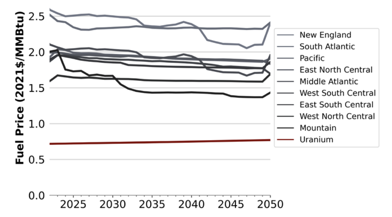
Input coal and uranium fuel prices used in Cambium 2022
Renewable fuel combustion turbines (RE-CT) are represented consistent with the Solar Futures Study (DOE 2021) and Cole et al. (2021). These RE-CT technologies have a renewably derived input fuel (e.g., hydrogen, biodiesel, ethanol, or green methane) that is assumed to cost $20/MMBtu in 2022 dollars at any point in time, in these scenarios. The additional electric load from the production of a renewably derived fuel is not incorporated into these scenarios.
The actual delivered cost that a renewably derived fuel could achieve is, highly uncertain. Current delivered prices for fuels like hydrogen are significantly higher than assumed here (e.g., the cost of delivering hydrogen via liquid tankers, not including production costs, was estimated at $68/MMBtu in 2021 dollars in 2020 (DOE 2020), although such delivery costs would be expected to decrease significantly if pipeline infrastructure were built). NREL’s Annual Technology Baseline (ATB) estimates that the delivered price of hydrogen could reach $56/MMBtu (in 2021 dollars) when using high temperature electrolysis in futures with high volume markets—although the ATB estimates do not include the incentives for hydrogen production in IRA, which can be as high as $22/MMBtu.
5.3 Generation and Capacity Metrics
Metric Family: total generation
Metric Name: generation Units: MWhbusbar
The generation metric reports the total generation from all generators within a region. It includes generation from storage (e.g., batteries or pumped hydropower storage). It does not include curtailed energy. If there are net imports or exports from a region, generation will not match load.
Behind-the-meter PV generation is included in the generation metric and is reported as the equivalent amount of busbar generation (i.e., it is increased to reflect the assumption that it does not incur distribution losses).
Metric Family: variable generation
Metric Name: variable_generation
Units: MWhbusbar
The variable_generation metric reports the total generation from all variable generators within a region, which includes PV, concentrating solar power (CSP) without storage, and wind. It does not include curtailed energy. Behind-the-meter PV generation is included, and as with generation, is reported as the equivalent amount of busbar generation.
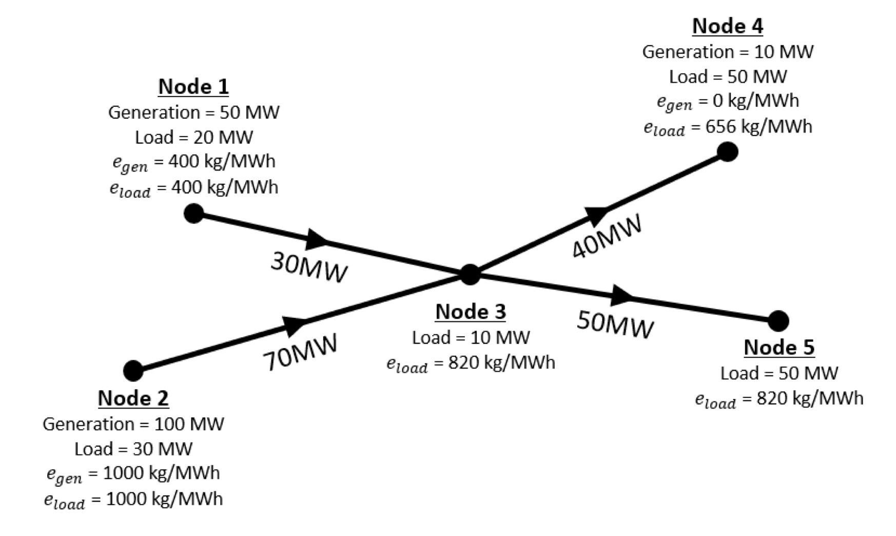
Simple Network Power Flow Coloring Chart
Four transmission lines. Only notes ????????1, ????????2, and ????????3 have generation, with emission rates for in- region generation (????????????????????????????????) of 400, 1,000, and 0 kg/MWh respectively. For this example, we assume there are no transmission losses.
The question we are trying to answer is: What is the emission rate that you could ascribe to each of the five nodes’ load (???????? ) For ????????1 and ????????2, the only power flowing into the node is from their own generation (they are not importing any power), and therefore we consider the emission rates induced by their load to be the rates of their in-region generation, which are 400 kg/MWh and 1,000 kg/MWh respectively.